Embedded Fuzzing Part 1: Getting Lauterbach snoops to Ghidra

This blog series introduces a joint research initiative between SCHUTZWERK and Lauterbach (as announced previously ), aimed at exploring debugger/tracer-guided fuzzing in embedded systems. The aim is to setup a dynamic fuzz testing framework using Ghidra (an open source reverse engineering tool) and Lauterbach Trace32®. Due to the excellent support of a wide range of microcontrollers and architectures provided by Lauterbach TRACE32®, the resulting fuzzing setup is aimed to be adaptable to most embedded systems with little effort.

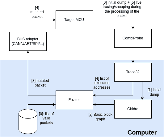
In the setup, the fuzzer uses the TRACE32® debugger to extract information (e.g. the program counter) from a target microcontroller or SoC at runtime [5] as well as an initial firmware dump [0]. This is used to optimize mutated input data that is sent to the attached target over data bus like CAN, Ethernet or RS232, as shown in Figure 1. Ghidra will be used to provide program flow information from the initial firmware dump to optimize the paths. Furthermore, Ghidra allows to identify useful program segments for instrumentation like privileged segments, dispatchers or crash handlers. This will be the main focus of this first blog post.

Additional Project Constraints

To get started we want to focus on setting up fuzzing with any hardware target with available JTAG debugging. This is a grey-box scenario where only the device is available, with no access to source code and no instrumentation compiled into the code, like often the case during embedded security assessments . In many cases, a trace port is not available either. Most production or pre-production devices are only equipped with minimal JTAG port for flashing.

Step 1: Program Flow Snooping

For scenarios where a tracing port on our target is not available, TRACE32® has the solution: Snooping. Using JTAG/SWD, TRACE32® periodically retrieves the Program Counter PC register of the target. Due to the comparably low speed of the JTAG/SWD interface and protocol overhead, the sample rate is relatively slow. Thus, we can only record a sparse set of PC register samples. To capture a higher number of PC values, the target processor’s clock speed may be reduced. This however will likely impact a real-world target’s application.

Using Lauterbach’s RCL API, we can automate TRACE32® from an external python application The automation can later be used to make repeated recordings and integrations for the fuzzer. To enable RCL, add/uncomment the following from your Lauterbach start configuration (usually called config.t32):

RCL=NETTCP
PORT=20000

In the following python example, we record PC samples of the target and save it to a file:

import time
import lauterbach.trace32.rcl as t32

dbg = t32.connect(node='localhost', port=20000, protocol="TCP")
cmd = dbg.cmd

print('Initializing the target...')
# Initialize your target here! e.g.:
# cmd('SYStem.CPU […]')
# cmd('SYStem.CONFIG.DEBUGPORTTYPE SWD')
# cmd('SYStem.JtagClock 32MHz') # Set the JTAG clock speed as high as possible
# …

cmd('SYStem.Up') # reset the target
print('Setting up debugger and snooper...')

snoop_freq = 50000 # This value can be set too high, it will be limited by the JTAG/SWD bandwidth
                   # At 32MHz SWD frequency, <50k samples/second were achieved.
snoop_rate = (1/snoop_freq) * (10**6)
cmd(f'SNOOPer.RATE {snoop_rate:1.3f}us')
snoop_duration = 3
sample_count = int(sample_duration * sample_freq * 1.1)
cmd(f'SNOOPer.SIZE {sample_count}.')
cmd('SNOOPer.Mode PC')

print(f'Running Program for {RUN_DURATION} seconds...')
cmd('Go')
time.sleep(RUN_DURATION) # The snooper will now collect samples
cmd('Break')

print(f'Saving snoop file to {SNOOPER_OUTPUT_PATH}...')
cmd('SNOOPer.OFF')
cmd(f'PRinTer.FILE {SNOOPER_OUTPUT_PATH}')
cmd('PRinTer.FileType CSV')
cmd('WinPrint.SNOOPer.List')

Due to the sparse sampling rate, the code of interest must be executed repeatedly to gain a meaningful sample set. For evaluation purposes, we iterate the object code in a loop. In real-world tests, we must repeatedly trigger the execution by other means.

The recorded samples are saved in a file at SNOOPER_OUTPUT_PATH in Lauterbach’s CSV format. In the next step, we’ll convert the file into the EZCOV format.

Step 2: Converting the snooped data to EZCOV

To analyze the recorded samples, we want to view it in the Ghidra Cartographer Plugin , which requires the samples to be in the EZCOV format. Lauterbach’s Snooper format and EZCOV are both CSV with one PC address in each line. The following python snippet converts the previously captured samples and saves it as EZCOV.

print(f'Converting Snoop file to EZCOV format...')
EZCOV_PATH = SNOOPER_OUTPUT_PATH + '.ezcov'

with open(SNOOPER_OUTPUT_PATH, 'r') as snoop_file:
	with open(EZCOV_PATH, 'w') as ezcov_file:
		ezcov_file.write('EZCOV VERSION: 1\n')
		while line := snoop_file.readline():
			columns = line.split(',')
			if len(columns) < 2: continue
			addr = columns[1].strip('"')
			if not addr.startswith('T:'): continue
			addr = addr.strip('T:')
		ezcov_file.write(f'0x{addr}, 4, [  ]\n')

print(f'Saved EZCOV file to {EZCOV_PATH}')

To implement any form of instrumentation, we first need to analyze the binary running on the microcontroller. To do this, we can dump the microcontroller’s memory and import it into Ghidra for analysis. Ghidra then decompiles the firmware. This serves two purposes: first, to generate a code flow graph that supports our fuzzer, and second, to visualize in ghidra-cartographer how the device behaves when it receives input.

Step 3: Dumping the target’s program memory

The extraction of the target’s firmware is different depending on the target. For a target with 1MiB of program flash at 0x8000000, a Lauterbach command such as the following would work.

Data.SAVE.IntelHex firmware.hex 0x8000000--0x800FFFFF

Step 4: Analyzing the snoop in Ghidra Cartographer

The firmware and snooped data can now be imported in Ghidra. Depending on the target, it may be necessary to offset the memory addresses when importing the firmware file to match the PC sample values.

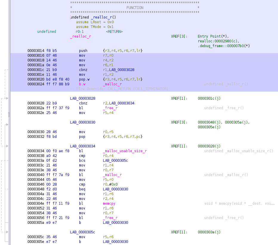
After importing the coverage data, code and instructions that have been executed will be highlighted, as shown above in Figure 2. Blank spots in-between two highlighted lines can be a result of the slow PC sampling rate or a jump instruction. Also, code blocks that have run less frequently may not be highlighted at all.

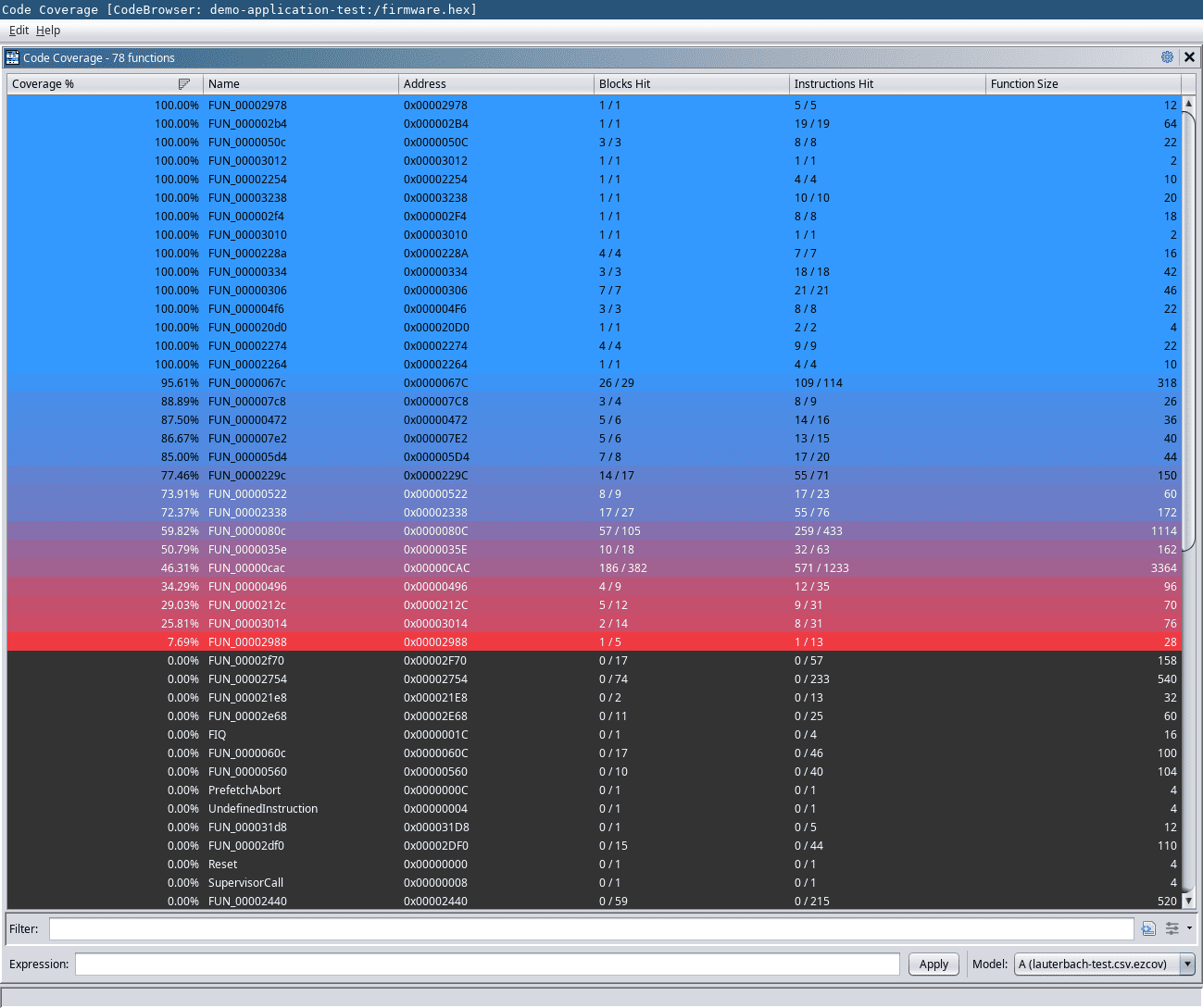
In the code coverage view of Cartographer (Figure 3), we can see coverage metrics for all functions. The table rows are colored as a heatmap, from fully covered functions (blue) to less covered functions (red). The Ghidra Cartographer plugin also offers additional options such as creating diffs of coverage samples and viewing multiple coverages simultaneously.

Using the Cartographer, we can now observe how the target behaves differently depending on different inputs. If we record PC samples while repeatedly feeding malformed data to the target, we may be able to observe error routines or crash handlers. Similarly, we can explore parts of the software such as password checks, privileged functions and shared functionality to further understand our target and find attack opportunities. This can be directly integrated on common Ghidra based reverse engineering workflows and allows getting around in large binaries much easier.

In the next article of this project we will take a look at how to put this setup in a fuzzing loop.