The previous blog post of the PROBoter series gave an insight on the automatic optical analysis for components mounted on the PCB. It introduced how the PROBoter attempts to localize all pins and components on the PCB.

This post focuses on the evaluation of voltage data measured on an operating PCB to gather information on the functionality and occurring communication. The list below gives an overview of the topics covered in this blog post series. The last link will be updated as soon as the corresponding part has been released.

• PROBoter demo video
• Part I: A platform for automated PCB analysis
• Part II: The PROBoter hardware platform
• Part III: Visual PCB analysis with Neural Networks and classic Computer Vision algorithms
• Part IV: Automated voltage signal analysis and protocol identification
• Part V: The PROBoter software framework

Time invariant protocol identification

Often, the missing knowledge about the communication protocols used on a Printed Circuit Board (PCB) is the only form of protection which prevents an attacker from decoding voltage signals into data for eavesdropping or injection of malicious data.

This article introduces the algorithm of the “Time Invariant Signal Analysis”, which the PROBoter uses to produce information on the functionality of the conducting paths identified on a PCB from passive eavesdropping. Using the gathered information, promising targets can be identified to perform a command injection or interact with a debug shell.

The algorithm is mainly based on a statistical analysis of the voltage signal, which makes the analysis time invariant. The determined characteristics are evaluated for the identification of the functionality, the data transmission protocol and, in case of UART and SPI, the transmission parameters.

Currently, the algorithm provides the following functionality:

1. Identification of a line’s functionality from its voltage data, e.g., ground, voltage supply, communication control, clock line or data transmission
2. Linking the datasets for synchronous data transmissions (consisting of a clock line and one or several data transmission lines)
3. Discerning four types of protocols:
   • UART
   • OneWire
   • I²C
   • SPI
4. Identification of the used data transmission parameters for the following protocols:
   • UART
     • Baud rate
     • Amount of data bits per frame
     • Amount of stop bits per frame
     • Usage of parity bit
     • Identification if the signal line is inverted
   • SPI
     • Identification of the clock polarity
     • Identification of the clock phase

The algorithm depends on frequent changes of the voltage states of the signals. Therefore, it works better with signals generated from real transmissions than signals based on theoretical edge cases with a low amount of changes.

The following sections guide the reader through the steps performed by the PROBoter platform, from the generation of data, used evaluation methods, identification of the functionality and protocols, finishing with the output of the analysis. For details on the algorithm, please see the original Master thesis with the title Algorithm for identification of bus protocols. [1].

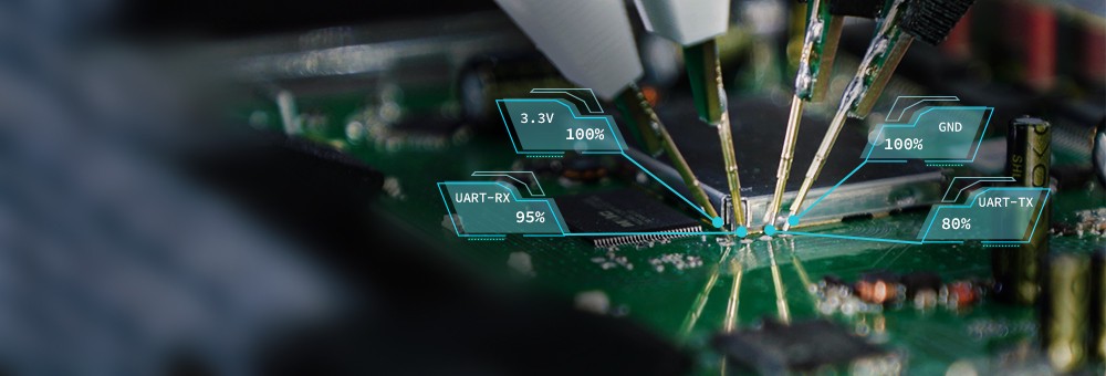
Data acquisition

For the identification of the protocols, the PROBoter has been equipped with a digital oscilloscope. The two analog input channels of the oscilloscope are connected to the measurement probes of the PROBoter, which allows the free positioning of the probes on the PCB and measurement of the voltages during operation. The duration and time resolution of the measurement is defined by user input. The start of each measurement is synced with the moment of supplying the target PCB with power. This allows a correlation of events for the measurement of several voltage lines.

For each measurement, the voltage data are stored as dataset in a list of values together with the time interval of the measurement. When all promising datasets were measured, the newly developed “Time Invariant Signal Analysis” algorithm starts the evaluation.

Evaluation of dataset characteristics

For each of the measured datasets, prominent characteristics are initially identified. This evaluation process is performed in three analysis steps:

• Determination of characteristics of the voltage distribution
• Determination of characteristics for the durations of voltage states (after noise removal by using filters)
  • Generation of histograms from the state durations
  • Performing a delta analysis
• Detection of repeating patterns

Subsequently, the algorithm uses these results to classify the functionality of the evaluated voltage signal, e.g.: ground, power supply or involved in data exchange.

Analysis of the Voltage Distribution

The first module of the algorithm uses the list of measured voltage levels to generate a histogram. From this it gets two characteristics for the voltage distribution:

1. The algorithm succeeds to identify the most common voltage levels. These should be identical to the levels of the upper and lower voltage for a binary voltage signal.
2. By the width of the voltage peaks, the algorithm gains information on the amount of voltage values around the upper and lower voltage level, and therefore the changing behavior for the voltage.

The amount and the width of the voltage peaks from the voltage histogram are first pieces of information which can be used for the identification of a voltage signal since they provide data on the most common voltage levels and change characteristics.

Comparing voltage distribution histograms

The following plot shows an exemplary voltage for an SPI transmission: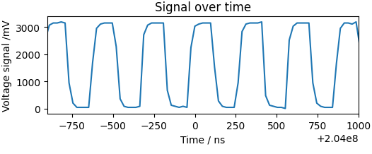

The resulting histogram of occurring voltages for the SPI transmission shows transition voltages between the two dominant voltage levels.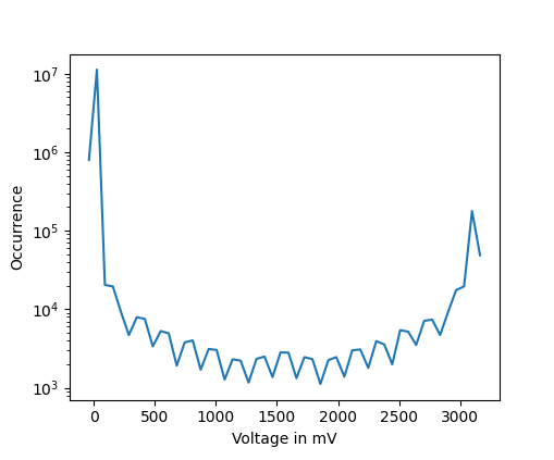

For comparison, the signal for an UART transmission shows a stronger distinction between low and high voltage states.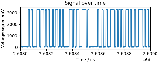

In the histogram, this leads to a low amount to no transition voltage values.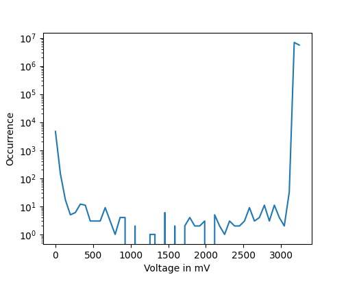

Event interval analysis

The second analysis step focuses on the evaluation of the durations of the voltage states. The algorithm identifies the moments for each voltage state change and calculates the durations of each state. Then, it uses this list of durations as input for the generation of histograms and a ‘delta analysis’. The following sections describe the process steps performed for the interval analysis.

Finding events

For finding moments of events at which the voltage signal changes from an upper to a lower voltage state or vice versa, the definition of Schmitt triggers is used. The Schmitt triggers are voltage limits set at 30% and 70% of the maximum voltage. When a voltage passes the 70% upwards or passes the 30% downward, the moment of passage shall act as significant trigger point.

Generation of List of Event Durations

To produce a statistical overview of voltage states durations, the algorithm marks each change of voltage state in a first run, producing an array of incidents, and calculates the time intervals and directions between two changes. The array comprises the shorter durations caused by signal activities as well as long durations caused by signal inactivity. The durations of inactivity can be larger than the durations of activity by several magnitudes while occurring more rarely.

This list (hereinafter referred to as ‘interval array’) presents the central source of information for the following two analysis mechanisms: Incident histograms and the delta analysis, which are described in the following sections below.

Generation of an Event Histogram

The algorithm produces histograms for single and for two consecutive voltage states (‘single incident histogram’ and ‘double incident histogram’).

Denoting a significant voltage change as an “event”, the time interval between two of these incidents are plotted along the horizontal axis in nanoseconds, while the amount of intervals which feature this duration, are plotted along the vertical axis. Voltage states which are followed by a voltage increase are plotted along the positive vertical axis, while the voltage states which are followed by a voltage decrease are plotted along the negative vertical axis.

The following is an incident histogram plot from a clock line which features high and low voltage states of quasi identical duration, leading to one significant peak for the positive and negative vertical axis each.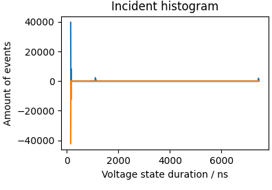

For comparison, the following is an incident histogram plot from a data transmission line, which features voltages states of varying durations.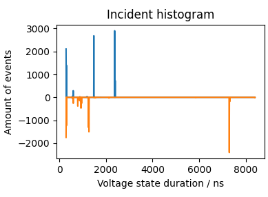

Finally, generating an incident histogram from the voltage data of a ground line does produce a noisy plot with high peaks for durations of $t ≈ 0~\mathrm{ns}$.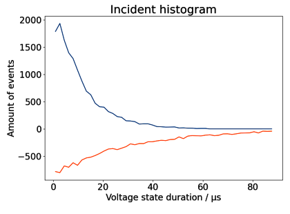

The first peak in the event histogram is a reoccurring significant duration. Usually, it is equivalent to the duration required to transmit a single bit. Thus, the duration at this first peak is expected to be the duration of one symbol.

For the generation of a double incident histogram, the durations of two consecutive entries of the interval array are used. This double incident histogram then shows the sum of two durations, which generates a single peak e.g., for clock signals or protocols based on Pulse Width Modulation (PWM).

The location and amount of peaks generate information about the repetition of events, which is used for the identification of the line’s functionality as well as the protocol type.

The delta analysis

The delta analysis is a newly developed time-invariant method for finding reoccurring duration patterns. It bases on the mathematical foundations of Min-Plus and Max-Plus calculus [2], which Thiele et al. use for their description of tasks arriving at and being processed by an embedded system [3].

The theory describes a sequence of arising events $r$ which occur within a time interval $[t, t + \Delta]$. Thus, the set of occurring events can be described as a function $r(t, t + \Delta)$. The minimum and maximum amount of events occurring within the interval $ \Delta $ can be enclosed by the two limiting functions $\alpha^u$ and $ \alpha^l $ for the upper and lower limit. Consequently: $$\alpha^l(t, t + \Delta) \le r(t, t + \Delta) \le \alpha^u (t, t + \Delta).$$

As shown in the following plot, identifying the minimum and maximum amount of events occurring within an increasing duration $\Delta t$, the amount of events increases when increasing the duration:

Mathematically, using a sliding window with the time interval $\delta^i$, $i=u,l$, the upper and lower amount of events $N^i$, $i=u,l$ found within this interval increases when the time interval gets increased.

For the PROBoter, the data contained in the interval array is used as input, since it contains the intervals between two changes of voltage states, which are also considered as events.

Plotting the data results in staircase functions with short steps for short intervals between changes and prolonged steps for intervals without change events. Prolonged steps repeating after an amount of shorter steps are a clue for a repeating pattern of transmission pauses.

The following is an exemplary plot of a SPI clock line which shows pauses between the transmission of data frames.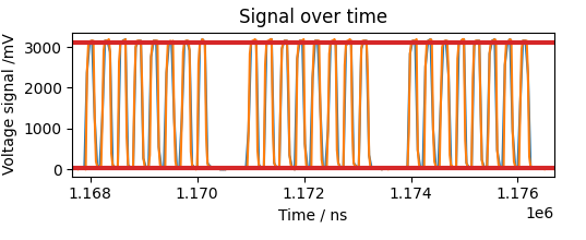

In the delta analysis plot below these lead to the prolonged steps in the delta analysis plot using the infimum amount of events: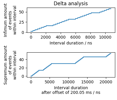

Pattern analysis

Some transmission protocols contain a repeating pattern which is used for synchronization between the communication partners. In case of the UART protocol, this pattern consists of one or two stop bit voltage-states followed by a start bit voltage state.

For a voltage signal, the occurrence of such a pattern can be unveiled by emphasizing the self-similarity of the signal. This is done by the autocorrelation function for a signal $r_{xx}$ consisting of $N$ values at index $m$: $$r_{xx}[m] = \frac{1}{N-|{m}|}\sum_{n=|m|}^{N-1}x[n]\ x[n-|m|]$$

A signal with an ideal repeating pattern creates high and regularly occurring peaks in the autocorrelation plot.

Larger datasets contribute to a better distinction between peaks and background noise as shown in the following exemplary autocorrelation plot for an UART transmission: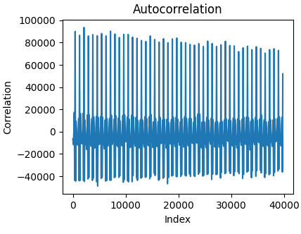

Identification of the signal type

For classifying the signal type for each dataset, the algorithm uses two sources of information: The extent of found voltage levels and the amount of reoccurring durations.

In total, the algorithm discerns five types of signals:

1. Signals with one elevated peak in the voltage histogram and only noise in the incident histogram usually occur for lines used as power supply.
2. Signals with a peak at a low voltage in the voltage histogram and only noise in the incident histogram, probably stem from a ground connection.
3. Signals with usually two peaks in the voltage histogram but no peaks in the incident histogram are considered as sporadic signals, which are used for communication control, as for deciding which partner is currently allowed to send messages on a data line.
4. Signals with usually two peaks in the voltage histogram and a single positive and negative peak each in the incident histogram are considered as periodic signals, as typical for clock signals.
5. Signals with usually two peaks in the voltage histogram and several peaks in the incident histogram are burst signals occurring often and irregularly, which are a typical behavior for the transmission of data.

Linking of datasets from synchronous data transmissions

For all the previously described analysis steps, the algorithm considered each dataset for itself. Since protocols like SPI and I²C do consist of a combination of a clock and data signals, the algorithm needs to link the involved datasets to a single signal group.

The algorithm uses two lists for the linking process: A list containing the identified clock signals, and a list containing the identified data signals.

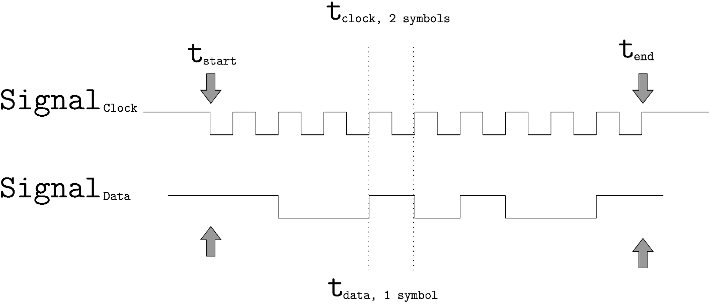
To test if a data and a clock signal were generated from the same transmission, the algorithm uses two pieces of information from each dataset:

1. The activities on the data line have to occur during the intervals of activities of the clock line,
2. The duration of a symbol on the data line has to be similar to the duration of one signal period on the clock line.

The data-datasets which have not been attributed to a synchronous transmission are expected to have been generated by an asynchronous transmission protocol, e.g., UART or OneWire.

Protocol Identification / Rating

To perform the protocol identification process, the algorithm compares the properties found in each signal group with a list of properties expected for each of the implemented protocol types (currently UART, OneWire, SPI and I²C).
The list of properties is based on the specifications of the used protocols. The properties used for the distinction of protocols are the:

• amount of involved datasets
• amount of dominant voltage levels
• occurring voltage range $U_{\mathrm{min}}$ … $U_{\mathrm{max}}$
• steepness of voltage state transitions
• data transmission speed
• maximum duration for occurring voltages during signal transmission
• duration of transmission blocks
• occurrence or absence of a repeating (synchronization) pattern
• check for symmetry of the durations of high and low voltage states
• check if the duration of voltage states are an integer multiple of the duration of one symbol

The following table shows an overview of characteristics of the protocols implemented in the algorithm together with characteristics of additional protocols, which are also popular in the automotive field.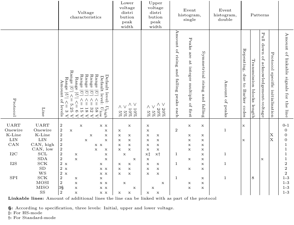

To identify the best fitting protocol, a counter is used. For each characteristic that is fulfilled by the measured data, the counter is increased; for each deviation, the value of the counter is reduced.

If a protocol is implemented to contain a data and a clock line, the algorithm tries to evaluate the properties for each measured dataset contained in a data group; for a missing dataset, the counter is reduced to prevent an identification as incomplete transmission protocol.

After each comparison, the counter result is stored. When the dataset has been compared with all known protocols, the algorithm returns all comparison counters.

Identification of Encoding Parameters

If the algorithm detects that the original encoding of a signal group is a UART or SPI protocol, the algorithm starts the respective module to identify the used transmission parameters.

Identification of the UART Protocol Parameters

In case of the UART protocol, the algorithm identifies the signal polarity, baud rate, frame length, amount of stop bits and parity bits. Since the quality of the identification strongly depends on the correct identification of the Start-Stop-bit pattern, a signal with a larger amount of changes generates more accurate results.

Polarity Inversion of Signal Line

Initially, the algorithm identifies the voltage state of the longest constant voltage. The algorithm expects that the voltage of the longest state is equivalent to the voltage of the default, inactive, voltage. In case of a non-inverted UART protocol, the voltage of the inactive state is expected to be logically high, while in case of a polarity inversion of a UART based transmission, the default voltage has to be logically low.

Identification of Baud Rate

The algorithm deduces the baud rate of the UART protocol based on the identified symbol duration of the dataset. For this purpose, it retrieves this information from getting the duration value of the first peak in the single event histogram.
For converting the symbol duration to the baud rate, the algorithm uses the inverse value of the duration, so that $$f_{\mathrm{baud}} = \frac{1}{t_{\mathrm{symbol}}}$$

The algorithm then rounds the calculated value to the next common baud rate before returning it to the user.

Amount of Stop Bits in UART

After having converted the voltage states into logical bits, the algorithm searches for the periodic occurrence of two types of patterns of logical bits in an interval of signal activity: bitpattern = b110 for an amount of two stop bits, and bitpattern = b10 for an amount of a single stop bit.

If either search for the patterns is successful, the algorithm expects to have found the correct pattern. If none of both patterns seem to occur regularly, the algorithm cannot identify the amount of stop bits. Therefore, it can neither determine the actual amount of bits in a frame nor the existence of a parity bit.

Check for Parity Bit Implementation

To determine if a parity bit is used for a UART signal, the algorithm converts the voltage signal into a sequence of logical bits first. Based on the information about the amount of used stop bits, it tests if the last voltage state between the start and stop bits appears to act as check bit for parity.

For an even parity, the combination of the last bit with the remaining bits of each evaluated frame shall be even. For odd parity, the total combination shall be odd.

Since transmission errors are common, if more than 90% of the evaluated data frames result as having an even or odd data bit, the function returns this result.

Amount of Data Bits per Frame

To calculate the amount of data bits per frame, the algorithm uses the original occurrence distance of the autocorrelation-pattern and subtracts the sum of identified start and stop bits as well as the existence of the parity bit, if any is used. Again, also this result of the evaluation is stored as property of the signal-group object.

Identification of the SPI Protocol Parameters

For the SPI protocol, there are only two parameters which are chosen before starting the transmission and generating a signal: The clock polarity and the clock phase.

Identification of Clock Polarity

The clock polarity defines whether the voltage of the clock signal is high or low during the inactive state. Therefore, similar to the identification of the polarity of the UART protocol described in the previous section, the clock polarity-function checks for the voltage of the longest duration without any activity. If this voltage is at the low voltage level, the returned clock polarity is polarity = 0, whereas if it is at the upper voltage, the returned clock polarity is polarity = 1.

Identification of Clock Phase

The clock phase characteristic describes at which edge of the clock signal the voltage state of the data signal is supposedly read out by the addressee component. Since the voltage signal of the data line is supposed to be stable around the timing of the voltage state evaluation, the edge for which the algorithm finds fewer changes probably is the edge for which the evaluation is triggered and therefore defines the clock phase. For this reason the algorithm checks the amount of voltage changes of the signal line which happen around the timings of the rising as well as around the falling edges of the clock line and stores those in lists each.
If the addressee reads the data at a falling clock edge, the clock phase CPHA = 1, while reading the voltage state at a rising clock edge, the clock phase CPHA = 0.

Generation of test data

For generating the data for development and testing the algorithm, two pieces of hardware were used: An USB-UART-converter to generate UART terminal signals, and an Arduino board which allowed the eavesdropping of voltage signals while the board accesses memory components which use the SPI and I²C protocol for data transmission. Additionally, the generation of voltage signals using the OneWire protocol has been implemented on the board.

For all protocols, messages with various lengths, transmission speeds and, where applicable, transmission parameters were generated and recorded for evaluation.

Evaluation Results

The algorithm correctly grouped and identified the protocols of 53 of the 54 prepared data set samples. The sample for which the identification algorithm fails to correctly identify the sample, is a long message transmitted at 500kBaud based on the UART protocol.

The failed identification is caused by a false linking of the UART-based sample to an SPI transmission. Yet, this mismatch is caused by a side effect when identifying larger amounts of datasets. If the algorithm only receives the datasets affected in the mismatch, it groups and identifies the involved datasets correctly.

Additionally, for a selected range of samples, the algorithm proves to correctly link the clock and data signals of 24 datasets, which only differ by variation in the offsets of start and end time.

For all of the 15 test-specific samples based on the UART protocol, the algorithm correctly identifies the existence and type of the parity bit, amount of stop bits and amount of data bits per frame. For all of the 18 test specific samples based on the UART protocol, it correctly identifies the baud rate used for the generation of the signal.

For SPI-based transmissions, samples without any modifications to the clock phase and polarity were generated. The algorithm correctly identifies the polarity for all of the 12 samples and the phase for 11 of the 12 samples.

In summary, the algorithm shows a reliable fully automatic identification and grouping for almost all the investigated dataset samples: The single case of wrong identification is only triggered if the affected sample is evaluated as part of a larger amount of samples. Therefore, the current influence of additional samples on the linking of signals has to be further investigated.

Outlook

Even though the identification algorithm is able to group and identify signals and their originating protocols, the current version of the algorithm can be further improved: Currently, the amount of processable data is limited due to an inflation of the data in the working memory. To improve the performance, the functions which currently demand much of the computer resources are planned to be optimized.

In extension to improving the processing performance, also the size of incoming and processed data can be reduced to increase the amount of processable datasets. This is planned to be achieved by a reduction of the resolution, measurement duration and, as far as it is possible, aggregating sequences of measurement data which show the same voltage levels: Currently, the algorithm runs blind measurements, without any information on the required measurement duration and resolution in time. Both pieces of information can be acquired based on the observation of voltage changes: The measurement duration can be defined on a minimum amount of changes required for running the statistical evaluation, and the resolution should be a certain multiple of the shortest time interval found between two changes of voltage states. This evaluation is not yet implemented so that resulting parameters could then be used as parameters for the actual measurement.

And finally, for extending the field of application of the algorithm, it shall be extended with the functionality to work out further characteristics of voltage signals. This allows the identification of additional signals based on protocols like the ones which are introduced in this blog post, but not implemented into the algorithm, yet.

Next Post

After the introduction to the signal analysis process, the upcoming post about the PROBoter software framework will provide an insight into the software components. This will cover the list of involved modules, their interfaces and functionality which is implemented in the project.

Follow us on Twitter , LinkedIn , Xing to stay up-to-date.

References / Credits

[1] Florian Schmid. Algorithm for identification of bus protocols , Masterthesis, Ruhr-Universität Bochum, Universitätsbibliothek, 2022.
[2] Raymond A Cuninghame-Green. Lecture Notes in Economics and Mathematical Systems, volume 166. Springer Science & Business Media, 1979.
[3] Lothar Thiele, Samarjit Chakraborty, and Martin Naedele. Real-time calculus for scheduling hard real-time systems. In 2000 IEEE International Symposium on Circuits and Systems (ISCAS), volume 4, pages 101–104. IEEE, 2000.

This work was sponsored by the BMBF project SecForCARs . We also want to thank igus GmbH for their support and providing hardware samples. The project was created at SCHUTZWERK GmbH (supervisors Dr. Bastian Könings & Msc. Heiko Ehret) in cooperation with the the Faculty of Computer Science at the Ruhr Universität Bochum (examiners Prof. Dr.-Ing. Christof Paar & M. Sc. Endres Puschner).

~ Florian Schmid